The Fourier Transform is one of the most important algorithms in signal processing. While there is a wealth of information out there on the topic, most of it seems focused solely on the math or optimized implementations of the algorithm. I have used this algorithm countless times in my research and thought I would share a programmers (and non-math major) perspective on the topic.
The Basic Transform
The Fourier transform is a mapping function that takes a series of samples (or function) in the time domain and maps them into the frequency domain. The transform is based on the Fourier Series, which is an expansion of a periodic function or signal into the sum of simpler sine and cosine functions.
![]()
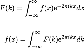
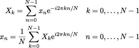
Looking at the example above, the periodic time data can be described as the sum of 4 sinusoidal functions with frequencies at 110, 220, 330, and 440 hz. So how does this mapping work? Unfortunately most descriptions of the Fourier transform (and its inverse) jump right into the following math with little explanation:
It is often difficult to grasp how we’re actually mapping from the time domain f(x) to the frequency domain F(k) (and vice versa) with these equations. To understand how this works, we need to look at some important properties about the spectrum analysis first. Let’s start by taking two periodic signals A and B, where A is our input signal and B is a signal we are generating:
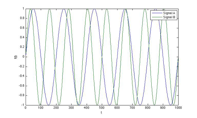
If we multiply these signals together and sum up the areas underneath the curves, we have:
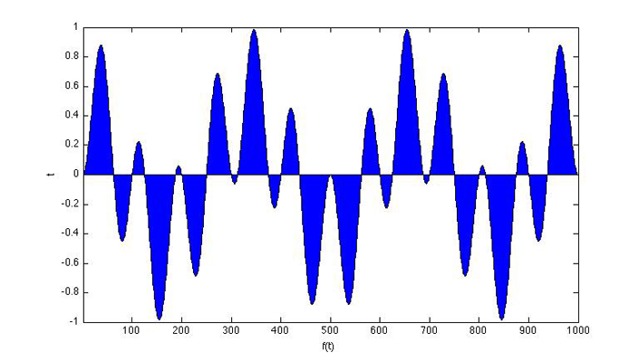
As you can see, about half the area is positive and the other half of the signal is negative and they will cancel each other out. However, if we multiply two signals together that share a frequency (say A x A), we’ll get:
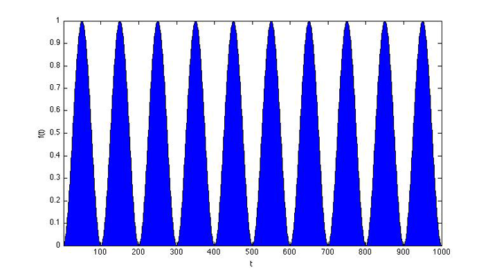
This tells us that our input signal has significant energy at the frequency of our test (generated) signal. If we extend this idea, sweeping from frequencies -∞ to ∞, we will end up with spikes (or Dirac δ functions) where our signals share frequencies and zero energy elsewhere. This is the basic idea behind Fourier transforms.
Working with Discrete Data
Since we are often working with small frames of sample data, we can’t actually test all frequencies from -∞ to ∞. The Discrete Fourier transform (DFT) is a modification of the Fourier transform that works with discrete sampled data. Our equations from above become:
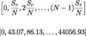
The DFT will test evenly spaced frequencies from 0 hz to the sampling frequency (Sr). For example, if we have a signal sampled at 44.1 kHz and 1024 samples N, the transform will test only the frequencies shown. The time complexity of the standard DFT is O(n2).
Making it Faster
In 1965, J.W. Cooley and John Turkey came up with a divide and conquer algorithm for calculating a Fast Fourier Transform (FFT) in O(n log n) time. To this day, this is the most widely used algorithm for Fourier transforms.
The Cooley-Turkey algorithm is often referred to as a radix-2 decimation-in-time (DIT) algorithm. The algorithm works by recursively splitting the data into smaller frames of size N/2 until you are calculating the FFT of a single value, which is the value itself. For this reason, the length of the input frames must be a power of 2. On each iteration, the data is split by even and odd indexes. This interleaving split is where the term “radix-2” comes from. The term “decimation-in-time” comes from the fact that we are splitting indexes that correspond to time.
Another important property of the DFT is that the outputs for 0 ≤ k < N/2 are identical to the outputs for N/2 ≤ k < N. Taking this into account, the above DFT algorithm can be split into the following:
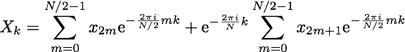
Note that for the odd terms, we were able to pull out the phase factor. This term is often referred to as the twiddle factor.
There are many implementations of the FFT in different languages. The fastest and most widely used implementation is FFTW, based on highly optimized C code. One interesting thing about FFTW is that the C code is actually generated by an OCaml program called ‘genfft’. In the next post, I’ll explore some implementations of the FFT in Scala.